1. 정밀도와 재현율의 트레이드 오프
1.1 Wine Data로 실습
1
2
3
4
5
6
7
8
9
import pandas as pd

wine_url = 'https://raw.githubusercontent.com/hmkim312/datas/main/wine/wine.csv'

wine = pd.read_csv(wine_url, index_col=0)
wine['taste'] = [1. if grade > 5 else 0. for grade in wine['quality']]

X = wine.drop(['taste','quality'],  axis = 1)
y = wine['taste']
- 정밀도와 재현율의 트레이드오프를 알아보기위해 와인 데이터로 해보도록 하겠다.
- 트레이드오프 : 객체의 어느 한부분의 품질을 높이거나 낮추는게, 다른 부분의 품질을 높이거나 낮추는데 영향을 끼치는 상황, 일반적으로 한쪽의 품질을 높이면, 다른쪽의 품질은 떨어지는 방향으로 흐름
1.2 데이터 분리
1
2
3
from sklearn.model_selection import train_test_split

X_train, X_test, y_train, y_test = train_test_split(X, y, test_size = 0.2, random_state = 13)
- 머신러닝에 적용하기위해 훈련용 데이터와 테스트용 데이터로 나눔
1.3 로지스틱 회귀 적용
1
2
3
4
5
6
7
8
9
10
11
from sklearn.linear_model import LogisticRegression
from sklearn.metrics import accuracy_score

lr = LogisticRegression(solver='liblinear', random_state=13)
lr.fit(X_train, y_train)

y_pred_tr = lr.predict(X_train)
y_pred_test = lr.predict(X_test)

print('Train Acc : ',accuracy_score(y_train, y_pred_tr))
print('Test Acc : ',accuracy_score(y_test, y_pred_test))
1
2
Train Acc :  0.7427361939580527
Test Acc :  0.7438461538461538
- 간단하게 로지스틱 회귀릘 적용하였고, 따로 전처리 및 파라미터 튜닝을 하지 않았으니, Accuracy는 0.74정도 나옴.
1.4 Classification Report
1
2
from sklearn.metrics import classification_report
print(classification_report(y_test, lr.predict(X_test)))
1
2
3
4
5
6
7
8
              precision    recall  f1-score   support

         0.0       0.68      0.58      0.62       477
         1.0       0.77      0.84      0.81       823

    accuracy                           0.74      1300
   macro avg       0.73      0.71      0.71      1300
weighted avg       0.74      0.74      0.74      1300
- classification_report는 데이터의 precision, recall, f1-score를 보여준다.
- precision, recall, f1-score는 링크 참조 https://hmkim312.github.io/posts/모델_평가/
1.5 Confusion Matrix
1
2
from sklearn.metrics import confusion_matrix
confusion_matrix(y_test, lr.predict(X_test))
1
2
array([[275, 202],
       [131, 692]])
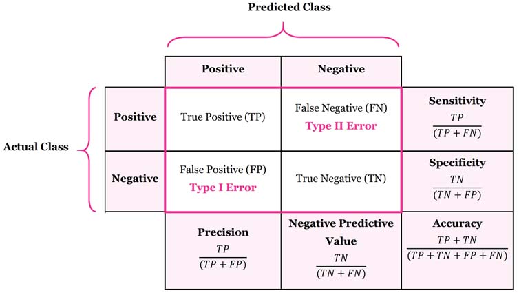
- 0번째 array가 0으로 예측한것 275 + 202 = 477
- 1번째 array가 1으로 예측한것 131 + 692 = 823
- [TP, FN]
[FP, TN]
1.6 Precision Recall Curve
1
2
3
4
5
6
7
8
9
10
11
import matplotlib.pyplot as plt
from sklearn.metrics import precision_recall_curve

plt.figure(figsize=(10, 8))
pred = lr.predict_proba(X_test)[:,1]
precision, recalls, thresholds = precision_recall_curve(y_test, pred)
plt.plot(thresholds, precision[:len(thresholds)], label = 'precision')
plt.plot(thresholds, recalls[:len(thresholds)], label = 'recall')
plt.grid()
plt.legend()
plt.show()
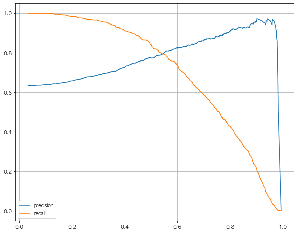
- Thresholds가 변함에 따라 recall과 Precision의 변화를 그래프로 그림
- Threshold : 임계값으로 0과 1을 나누는 수치
- Recall이 중요하면 Threshold를 낮게 설정, Precision이 중요하면 Threshold를 높게 설정함
1.7 threshold = 0.5
1
2
pred_proba = lr.predict_proba(X_test)
pred_proba[:3]
1
2
3
array([[0.40552193, 0.59447807],
       [0.50938053, 0.49061947],
       [0.10223984, 0.89776016]])
- 위의 그래프 상으로 Threshold를 0.5 부근으로 로 두는게 recall과 precision이 가깝게 된다.
- Recall과 Precision중 무엇이 중요한지는 데이터애 따라 다르니, 잘 결정해야함
1.8 간단히 확인해보기
1
2
3
import numpy as np

np.concatenate([pred_proba, y_pred_test.reshape(-1, 1)], axis=1)
1
2
3
4
5
6
7
array([[0.40552193, 0.59447807, 1.        ],
       [0.50938053, 0.49061947, 0.        ],
       [0.10223984, 0.89776016, 1.        ],
       ...,
       [0.22560159, 0.77439841, 1.        ],
       [0.67382439, 0.32617561, 0.        ],
       [0.31446618, 0.68553382, 1.        ]])
1.9 Threshold 바꿔보기 - Binarizer
1
2
3
4
5
from sklearn.preprocessing import Binarizer

binarizer = Binarizer(threshold=0.6).fit(pred_proba)
pred_bin = binarizer.transform(pred_proba)[:,1]
pred_bin
1
array([0., 0., 1., ..., 1., 0., 1.])
- Binarizer를 사용하여 Threshold를 0.6으로 잡고, 그 이하는 0 이상은 1로 바꿈
1.10 다시 Classification Report
1
print(classification_report(y_test, pred_bin))
1
2
3
4
5
6
7
8
              precision    recall  f1-score   support

         0.0       0.62      0.73      0.67       477
         1.0       0.82      0.74      0.78       823

    accuracy                           0.73      1300
   macro avg       0.72      0.73      0.72      1300
weighted avg       0.75      0.73      0.74      1300
- classification_report를 사용하여 report 확인
1.11 Confusion Matrix
1
confusion_matrix(y_test, pred_bin)
1
2
array([[348, 129],
       [216, 607]])
- 아까와 비교하여 threshold가 바뀌어서 recall, precision의 수치가 바뀜