1. Olivetti 데이터
1.1 데이터 소개
- 미국의 AT&T와 캠프리지 대학 전산 연구실에서 공동으로 제작한 얼굴 사진 데이터
- 얼굴 인식 등 다양한 분야에서 활용되고 있음
- 일부 데이터가 sklearn에 dataset으로 내장되어 있음
2. 실습
2.1 Data load
1
2
3
4
from sklearn.datasets import fetch_olivetti_faces

faces_all = fetch_olivetti_faces()
print(faces_all.DESCR)
1
2
3
4
5
6
7
8
9
10
11
12
13
14
15
16
17
18
19
20
21
22
23
24
25
26
27
28
29
30
31
32
33
34
35
36
37
38
39
40
41
42
43
44
.. _olivetti_faces_dataset:

The Olivetti faces dataset
--------------------------

`This dataset contains a set of face images`_ taken between April 1992 and
April 1994 at AT&T Laboratories Cambridge. The
:func:`sklearn.datasets.fetch_olivetti_faces` function is the data
fetching / caching function that downloads the data
archive from AT&T.

.. _This dataset contains a set of face images: http://www.cl.cam.ac.uk/research/dtg/attarchive/facedatabase.html

As described on the original website:

    There are ten different images of each of 40 distinct subjects. For some
    subjects, the images were taken at different times, varying the lighting,
    facial expressions (open / closed eyes, smiling / not smiling) and facial
    details (glasses / no glasses). All the images were taken against a dark
    homogeneous background with the subjects in an upright, frontal position
    (with tolerance for some side movement).

**Data Set Characteristics:**

    =================   =====================
    Classes                                40
    Samples total                         400
    Dimensionality                       4096
    Features            real, between 0 and 1
    =================   =====================

The image is quantized to 256 grey levels and stored as unsigned 8-bit
integers; the loader will convert these to floating point values on the
interval [0, 1], which are easier to work with for many algorithms.

The "target" for this database is an integer from 0 to 39 indicating the
identity of the person pictured; however, with only 10 examples per class, this
relatively small dataset is more interesting from an unsupervised or
semi-supervised perspective.

The original dataset consisted of 92 x 112, while the version available here
consists of 64x64 images.

When using these images, please give credit to AT&T Laboratories Cambridge.
- 올리베티 데이터의 일부만 이용하여 PCA 실습 진행
2.2 특정 샘플을 선택 후 출력
1
2
3
4
5
6
7
8
9
10
11
12
13
14
15
16
17
18
19
20
21
import matplotlib.pyplot as plt

K = 20
faces = faces_all.images[faces_all.target == K]

N = 2
M = 5

fig = plt.figure(figsize=(10, 5))
plt.subplots_adjust(top = 1, bottom = 0, hspace= 0, wspace= 0.05)

for n in range(N * M):
    ax = fig.add_subplot(N , M, n + 1)
    ax.imshow(faces[n], cmap = plt.cm.bone)
    ax.grid(False)
    ax.xaxis.set_ticks([])
    ax.yaxis.set_ticks([])

plt.suptitle('Olivetti')
plt.tight_layout()
plt.show()
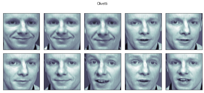
- K값을 변환하면 다른 사람의 얼굴이 나온다
- 양옆을 보는 사진, 웃는 사진 등 1명이 10장으로 구성되어있음
2.3 두개의 성분으로 분석
1
2
3
4
5
6
7
8
9
10
from sklearn.decomposition import PCA

K = 20

pca = PCA(n_components= 2)

X = faces_all.data[faces_all.target == K]
W = pca.fit_transform(X)

X_inv = pca.inverse_transform(W)
2.4 PCA 후 해당 데이터로 원점으로 복귀한 데이터로 그린 이미지
1
2
3
4
5
6
7
8
9
10
11
12
13
14
15
16
N = 2
M = 5

fig = plt.figure(figsize=(10, 5))
plt.subplots_adjust(top=1, bottom=0, hspace=0, wspace=0.05)

for n in range(N * M):
    ax = fig.add_subplot(N, M, n + 1)
    ax.imshow(X_inv[n].reshape(64, 64), cmap=plt.cm.bone)
    ax.grid(False)
    ax.xaxis.set_ticks([])
    ax.yaxis.set_ticks([])

plt.suptitle('PCA result')
plt.tight_layout()
plt.show()
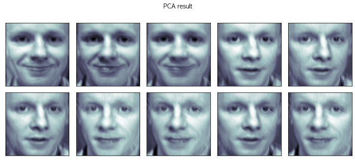
- PCA를 진행 한 데이터로 원점으로 복귀(X_inv = pca.inverse_transform(W))로 그린 사진으로, 원래의 데이터랑 큰 차이가 없는것으로 보인다
2.5 원점과 두 개의 eigen face
1
2
3
4
5
6
7
8
9
10
11
12
13
14
15
face_mean = pca.mean_.reshape(64, 64)
face_p1 = pca.components_[0].reshape(64, 64)
face_p2 = pca.components_[1].reshape(64, 64)

plt.figure(figsize=(12, 7))
plt.subplot(131)
plt.imshow(face_mean, cmap=plt.cm.bone)
plt.grid(False); plt.xticks([]); plt.yticks([]); plt.title('mean')
plt.subplot(132)
plt.imshow(face_p1, cmap=plt.cm.bone)
plt.grid(False); plt.xticks([]); plt.yticks([]); plt.title('face_p1')
plt.subplot(133)
plt.imshow(face_p2, cmap=plt.cm.bone)
plt.grid(False); plt.xticks([]); plt.yticks([]); plt.title('face_p2')
plt.show()
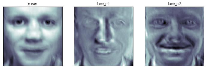
- face_mean은 원점, face_p1은 한방향, face_p2은 다른 한방향으로 생각하면 된다.
- 이 3개의 이미지가 앞에서 보았던 10개의 이미지를 대표한다고 생각하면 된다
2.5 가중치 선정
1
2
3
4
5
6
import numpy as np

N = 2
M = 5
w = np.linspace(-5, 10, N * M)
w
1
2
array([-5.        , -3.33333333, -1.66666667,  0.        ,  1.66666667,
        3.33333333,  5.        ,  6.66666667,  8.33333333, 10.        ])
- -5 ~ 10까지 가중치(w)를 설정하여 face에 적용시켜보려고 한다
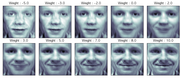
2.6 첫번째 성분의 변화
1
2
3
4
5
6
7
8
9
10
11
12
fig = plt.figure(figsize=(10, 5))
plt.subplots_adjust(top = 1, bottom= 0, hspace=0, wspace= 0.05)

for n in range(N * M):
    ax = fig.add_subplot(N, M, n + 1)
    ax.imshow(face_mean + w[n] * face_p1, cmap=plt.cm.bone)
    plt.grid(False); plt.xticks([]); plt.yticks([])
    plt.title('Weight : ' + str(round(w[n])))


plt.tight_layout()
plt.show()
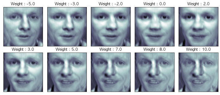
- 평균얼굴(원점)에 가중치를 곱한 face_p1을 더하면 해당 얼굴이 보인다. 오른쪽과 왼쪽을 보는 얼굴로 파악된다
2.7 두번째 성분에 대한 변화
1
2
3
4
5
6
7
8
9
10
11
12
fig = plt.figure(figsize=(10, 5))
plt.subplots_adjust(top = 1, bottom= 0, hspace=0, wspace= 0.05)

for n in range(N * M):
    ax = fig.add_subplot(N, M, n + 1)
    ax.imshow(face_mean + w[n] * face_p2, cmap=plt.cm.bone)
    plt.grid(False); plt.xticks([]); plt.yticks([])
    plt.title('Weight : ' + str(round(w[n])))


plt.tight_layout()
plt.show()
- 두번째 얼굴은 정면을 바라보고 있고, 가중치가 더해짐에 따라 점점 무표정이 되거나 웃는 얼굴로 변화되는것으로 파악된다
2.8 두개의 성분을 모두 표현하기
1
2
3
4
nx, ny = (5, 5)
x = np.linspace(-5, 8, nx)
y = np.linspace(-5, 8, ny)
w1, w2 = np.meshgrid(x, y)
2.9 Shpae 조정
1
w1.shape
1
(5, 5)
- shape가 5 ,5로 되어있으므로, 이를 조정하여 25로 바꾼다
1
2
3
w1 = w1.reshape(-1, )
w2 = w2.reshape(-1, )
w1.shape
1
(25,)
2.10 성분 2개에 가중치를 준것을 출력
1
2
3
4
5
6
7
8
9
10
11
12
fig = plt.figure(figsize=(12, 10))
plt.subplots_adjust(top=1, bottom=0, hspace=0, wspace=0.05)

N = 5
M = 5

for n in range(N * M):
    ax = fig.add_subplot(N, M, n+1)
    ax.imshow(face_mean + w1[n] * face_p1 + w2[n] * face_p2, cmap = plt.cm.bone)
    plt.grid(False); plt.xticks([]); plt.yticks([])
    plt.title('Weight : ' + str(round(w1[n],1)) + ', ' + str(round(w2[n],1)))
plt.show()
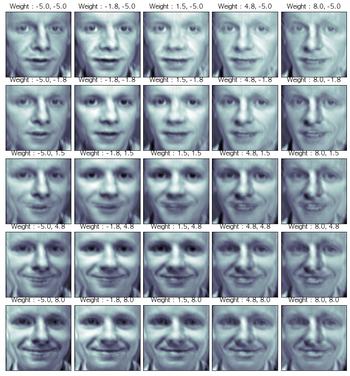
- 위의 사진들은 원점(평균얼굴)에서 성분1과 성분2의 사이들에 퍼저있는 사진이라고 생각하면됨
- 앞에서 K값을 변경하면 다른 사람들의 얼굴이 나오고, 해당 얼굴로도 PCA를 해보면 정면, 좌우가 아닌 다른 성분으로 분리된 사진들이 나오게 된다.