1. MNIST
1.1 MNIST Data
- NIST는 미국 국립표준기술연구소(National Institute of Standards and Technology)의 약자입니다. 여기서 진행한 미션 중에 손글씨 데이터를 모았는데, 그중 숫자로 된 데이터를 MNIST라고 합니다.
- 28 * 28 픽셀의 0 ~ 9 사이의 숫자 이미지와 레이블로 구성된 데이터 셋
- 머신러닝 공부하는 사람들이 입문용으로 사용을 많이함
- 60000개의 훈련용 셋과 10000개의 실험용 셋트로 구성되어있음
- 데이터는 kaggle에 있습니다. https://www.kaggle.com/oddrationale/mnist-in-csv
2. 실습
2.1 Data Load
1
2
3
4
5
6
import tensorflow as tf

mnist = tf.keras.datasets.mnist

(x_train, y_train), (x_test, y_test) = mnist.load_data()
x_train, x_test = x_train / 255.0, x_test / 255.0
1
2
Downloading data from https://storage.googleapis.com/tensorflow/tf-keras-datasets/mnist.npz
11493376/11490434 [==============================] - 2s 0us/step
- MNIST 데이터는 텐서플로우에 내장되어있다.
- 각 사진의 픽셀의 최대값이 255값이여서, 0 ~ 1 사이의 값으로 조정함 (Min Max Scaler)
2.2 One Hot Encoding
- 라벨값이 0 ~ 9로 되어있기 떄문에 사실은 One Hot Encoding을 해야함
- 하지만 텐서플로우의 Loss 함수를 Sparse Categorical Crossentropy로 설정하면 같은 효과가 나옴
- 그래서 따로 One Hot Encoding은 하지 않음
2.3 모델의 구성도
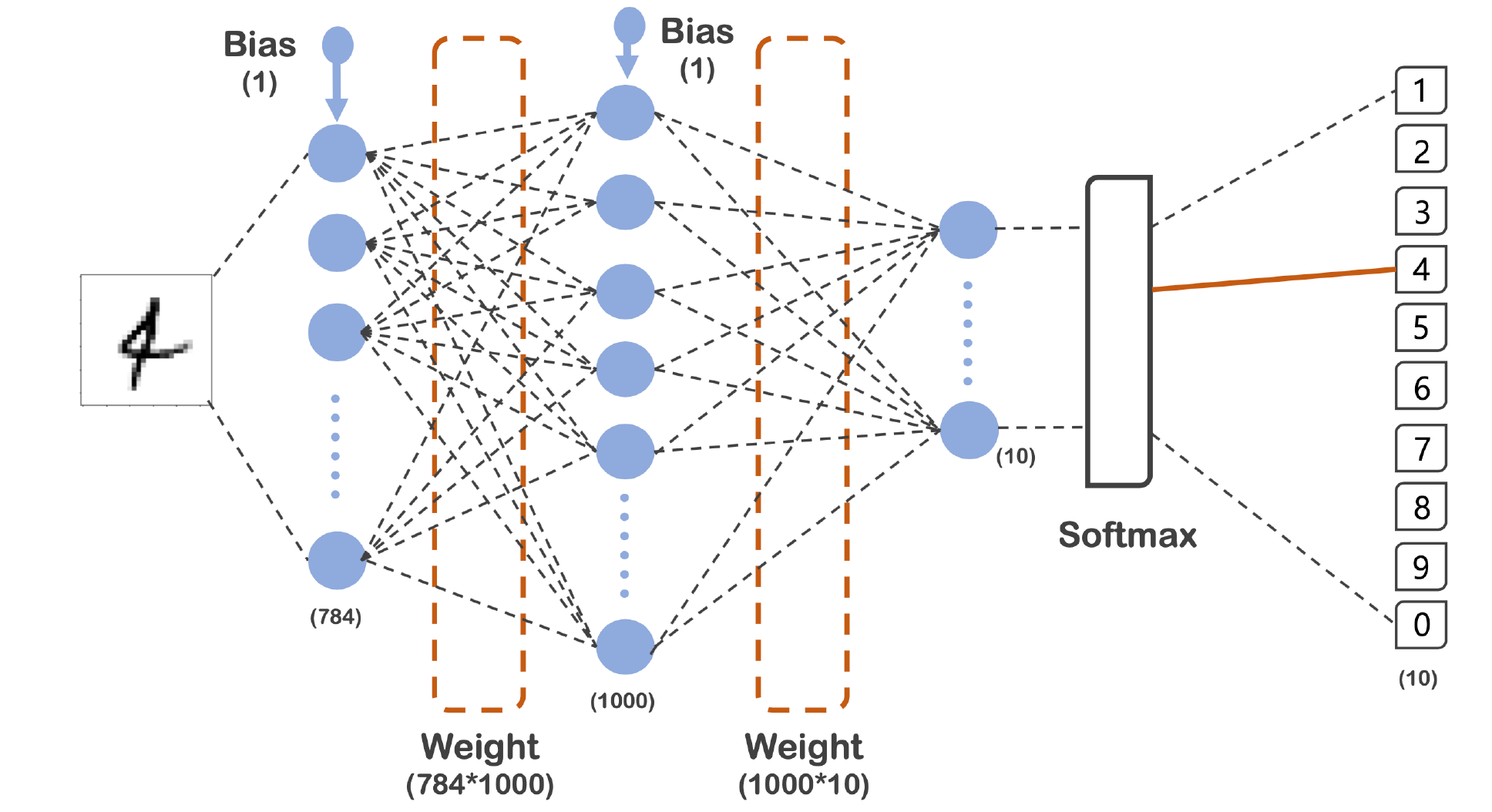
- 784 -> 1000 -> 10
- 784는 28픽셀 * 28픽셀로 나온 숫자이다.
- 마지막은 0 ~ 9까지의 타겟이므로 10개
- 총 3개의 레이어를 지나고 Output이 나오는것
2.4 모델 생성
1
2
3
4
5
6
7
model = tf.keras.models.Sequential([
    tf.keras.layers.Flatten(input_shape = (28,28)),
    tf.keras.layers.Dense(1000, activation = 'relu'),
    tf.keras.layers.Dense(10, activation = 'softmax')
])

model.compile(optimizer = 'adam', loss = 'sparse_categorical_crossentropy', metrics = ['accuracy'])
- 활성화 함수는 relu와 sotfmax를 사용
- 최적화는 adam, Loss는 아까 이야기했던 sparse categorical crossentropy로 하고 평가는 accuracy로 하였음
2.5 Softmax

- Softmax 클래스 분류 문제를 풀 때 점수 벡터를 클래스 별 확률로 변환하기 위해 흔히 사용하는 함수
- 각 점수 벡터에 지수를 취한 후, 정규화 상수로 나누어 총 합이 1이 되도록 계산됨
2.6 Model Summary
1
model.summary()
1
2
3
4
5
6
7
8
9
10
11
12
13
14
Model: "sequential"
_________________________________________________________________
Layer (type)                 Output Shape              Param #
=================================================================
flatten (Flatten)            (None, 784)               0
_________________________________________________________________
dense (Dense)                (None, 1000)              785000
_________________________________________________________________
dense_1 (Dense)              (None, 10)                10010
=================================================================
Total params: 795,010
Trainable params: 795,010
Non-trainable params: 0
_________________________________________________________________
- 모델의 구성도와 코드의 summary가 동일한지 확인해야함
2.7 Fit
1
2
3
4
5
6
7
import time

start_time = time.time()
hist = model.fit(x_train, y_train, validation_data=(x_test, y_test),
                 epochs=10, batch_size=100, verbose=1)

print(f'Fit time : {time.time() - start_time}')
1
2
3
4
5
6
7
8
9
10
11
12
13
14
15
16
17
18
19
20
21
Epoch 1/10
600/600 [==============================] - 2s 3ms/step - loss: 0.2232 - accuracy: 0.9343 - val_loss: 0.1175 - val_accuracy: 0.9659
Epoch 2/10
600/600 [==============================] - 2s 3ms/step - loss: 0.0860 - accuracy: 0.9748 - val_loss: 0.0770 - val_accuracy: 0.9767
Epoch 3/10
600/600 [==============================] - 2s 3ms/step - loss: 0.0537 - accuracy: 0.9840 - val_loss: 0.0774 - val_accuracy: 0.9752
Epoch 4/10
600/600 [==============================] - 2s 3ms/step - loss: 0.0364 - accuracy: 0.9888 - val_loss: 0.0780 - val_accuracy: 0.9749
Epoch 5/10
600/600 [==============================] - 2s 3ms/step - loss: 0.0268 - accuracy: 0.9916 - val_loss: 0.0666 - val_accuracy: 0.9787
Epoch 6/10
600/600 [==============================] - 2s 3ms/step - loss: 0.0192 - accuracy: 0.9942 - val_loss: 0.0595 - val_accuracy: 0.9813
Epoch 7/10
600/600 [==============================] - 2s 3ms/step - loss: 0.0130 - accuracy: 0.9961 - val_loss: 0.0623 - val_accuracy: 0.9810
Epoch 8/10
600/600 [==============================] - 2s 4ms/step - loss: 0.0131 - accuracy: 0.9960 - val_loss: 0.0697 - val_accuracy: 0.9797
Epoch 9/10
600/600 [==============================] - 2s 3ms/step - loss: 0.0125 - accuracy: 0.9961 - val_loss: 0.0725 - val_accuracy: 0.9807
Epoch 10/10
600/600 [==============================] - 2s 3ms/step - loss: 0.0072 - accuracy: 0.9980 - val_loss: 0.0712 - val_accuracy: 0.9804
Fit time : 19.54804039001465
- 총 10번의 Epochs를 하여 학습 총 20초 정도 걸림
2.8 Acc와 Loss 그리기
1
2
3
4
5
6
7
8
9
10
import matplotlib.pyplot as plt

plot_target = ['loss', 'val_loss', 'accuracy', 'val_accuracy']
plt.figure(figsize=(12, 8))

for each in plot_target:
    plt.plot(hist.history[each], label = each)
plt.legend()
plt.grid()
plt.show()
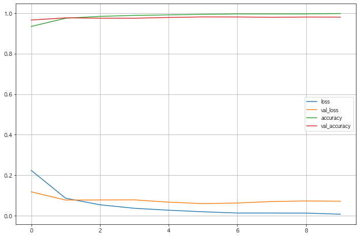
- 과적합 등 우려되는 상황은 보이지않는다, 또한 Loss도 잘 떨어지는것으로 확인
2.9 Accuracy 확인
1
2
3
score = model.evaluate(x_test, y_test)
print('Test loss : ', score[0])
print('Test Accuracy : ', score[1])
1
2
3
313/313 [==============================] - 0s 867us/step - loss: 0.0712 - accuracy: 0.9804
Test loss :  0.07119151949882507
Test Accuracy :  0.980400025844574
- Accuracy가 0.98나옴
- 이전에 했던 https://hmkim312.github.io/posts/MNIST로_해보는_PCA와_kNN/에서 0.94가 나왔었는데, 더 잘나옴
2.10 예측
1
2
3
4
5
import numpy as np

predicted_result = model.predict(x_test)
predicted_labels = np.argmax(predicted_result, axis = 1)
predicted_labels[:10], y_test[:10]
1
2
(array([7, 2, 1, 0, 4, 1, 4, 9, 5, 9]),
 array([7, 2, 1, 0, 4, 1, 4, 9, 5, 9], dtype=uint8))
- predicted_labels : 예측한 데이터
- y_test : 실제 데이터
2.11 틀린 데이터만
1
2
3
4
5
6
wrong_result = []

for n in range(0, len(y_test)):
    if predicted_labels[n] != y_test[n]:
        wrong_result.append(n)
len(wrong_result)
1
196
- 총 1만개 중 196개의 데이터가 틀렸다
2.12 그중 16개만 랜덤으로 뽑기
1
2
3
4
import random

samples = random.choices(population= wrong_result, k = 16)
samples
1
2
3
4
5
[2135,
 5450,
 ...
 6641,
 4176]
2.13 틀린 데이터 눈으로 확인
1
2
3
4
5
6
7
8
9
plt.figure(figsize=(14, 12))

for idx, n in enumerate(samples):
    plt.subplot(4, 4, idx + 1)
    plt.imshow(x_test[n].reshape(28, 28), cmap = 'Greys', interpolation='nearest')
    plt.title('Label : ' + str(y_test[n]) + ' Predict : ' + str(predicted_labels[n]))
    plt.axis('off')

plt.show()
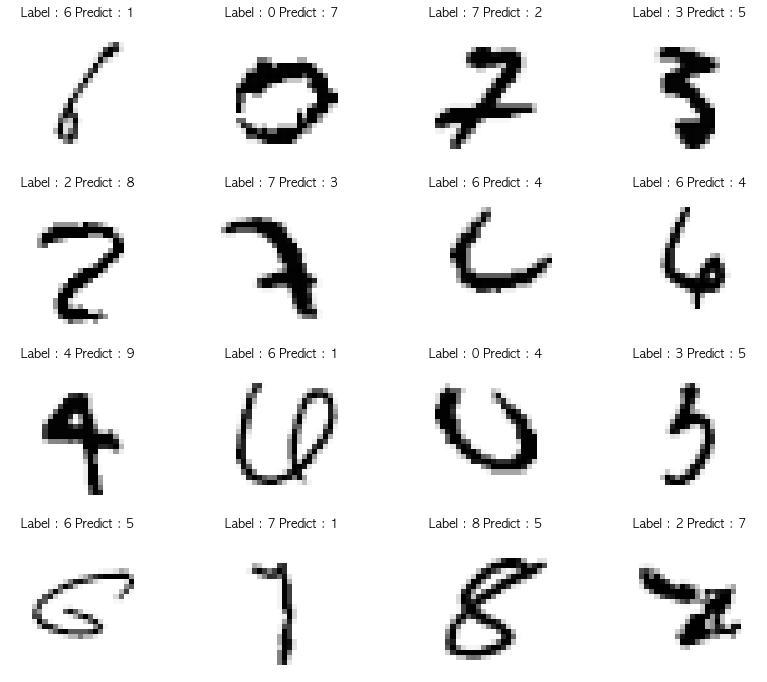
- 실제로 헷갈리는것들도 보인다. 틀릴만 한듯
3. MNIST Fashion
3.1 MINIST Fashion Data
- 숫자로된 MNIST Data 처럼 28 * 28 크기의 패션과 관련된 10개 종류의 데이터임
- 레이블 설명
1
2
3
4
5
6
7
8
9
10
0 티셔츠/탑
1 바지
2 풀오버(스웨터의 일종)
3 드레스
4 코트
5 샌들
6 셔츠
7 스니커즈
8 가방
9 앵클 부츠
3.2 Data Load
1
2
3
4
5
6
import tensorflow as tf

fashion_mnist = tf.keras.datasets.fashion_mnist

(X_train, y_train), (X_test, y_test) = fashion_mnist.load_data()
X_train, X_test = X_train / 255.0, X_test / 255.0
1
2
3
4
5
6
7
8
Downloading data from https://storage.googleapis.com/tensorflow/tf-keras-datasets/train-labels-idx1-ubyte.gz
32768/29515 [=================================] - 0s 0us/step
Downloading data from https://storage.googleapis.com/tensorflow/tf-keras-datasets/train-images-idx3-ubyte.gz
26427392/26421880 [==============================] - 7s 0us/step
Downloading data from https://storage.googleapis.com/tensorflow/tf-keras-datasets/t10k-labels-idx1-ubyte.gz
8192/5148 [===============================================] - 0s 0us/step
Downloading data from https://storage.googleapis.com/tensorflow/tf-keras-datasets/t10k-images-idx3-ubyte.gz
4423680/4422102 [==============================] - 3s 1us/step
- MNIST Fashoin 데이터도 텐서플로우에 있음
- 아까와 마찬가지로 최대 255 숫자로 되어있어서, 0과 1사이로 만들기위해 255로 나눠줌
3.3 데이터 확인
1
2
3
4
5
6
7
8
9
10
11
12
13
import random
import matplotlib.pyplot as plt

samples = random.choices(population=range(0, len(y_train)), k = 16)
plt.figure(figsize=(14, 12))

for idx, n in enumerate(samples):
    plt.subplot(4, 4, idx+1)
    plt.imshow(X_train[n].reshape(28, 28), cmap = 'Greys', interpolation='nearest')
    plt.title('Label : ' + str(y_train[n]))
    plt.axis('off')

plt.show()
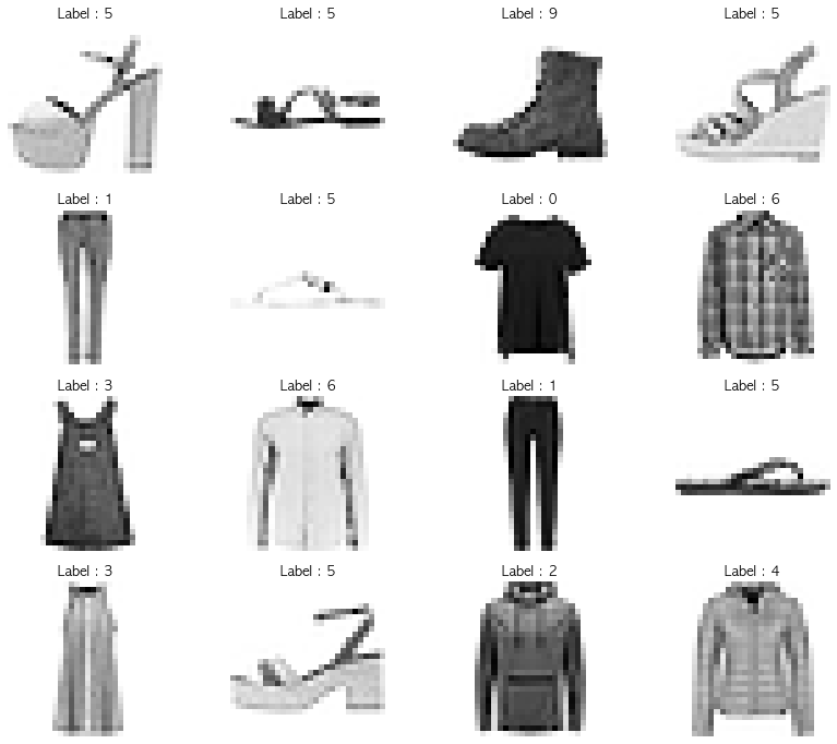
- 레이블 설명
1
2
3
4
5
6
7
8
9
10
0 티셔츠/탑
1 바지
2 풀오버(스웨터의 일종)
3 드레스
4 코트
5 샌들
6 셔츠
7 스니커즈
8 가방
9 앵클 부츠
3.4 모델생성
1
2
3
4
5
6
7
model = tf.keras.models.Sequential([
    tf.keras.layers.Flatten(input_shape = (28,28)),
    tf.keras.layers.Dense(1000, activation = 'relu'),
    tf.keras.layers.Dense(10, activation = 'softmax')
])

model.compile(optimizer = 'adam', loss = 'sparse_categorical_crossentropy', metrics = ['accuracy'])
- 모델은 숫자 데이터 할떄와 동일하게 생성
3.5 Summary
1
model.summary()
1
2
3
4
5
6
7
8
9
10
11
12
13
14
Model: "sequential_1"
_________________________________________________________________
Layer (type)                 Output Shape              Param #
=================================================================
flatten_1 (Flatten)          (None, 784)               0
_________________________________________________________________
dense_2 (Dense)              (None, 1000)              785000
_________________________________________________________________
dense_3 (Dense)              (None, 10)                10010
=================================================================
Total params: 795,010
Trainable params: 795,010
Non-trainable params: 0
_________________________________________________________________
- 모델의 구성도와 Summary가 같은지 확인
3.6 Fit
1
2
3
4
5
6
7
import time

start_time = time.time()
hist = model.fit(X_train, y_train, validation_data=(X_test, y_test),
                 epochs=10, batch_size=100, verbose=1)

print(f'Fit time : {time.time() - start_time}')
1
2
3
4
5
6
7
8
9
10
11
12
13
14
15
16
17
18
19
20
21
Epoch 1/10
600/600 [==============================] - 2s 4ms/step - loss: 0.4895 - accuracy: 0.8250 - val_loss: 0.4100 - val_accuracy: 0.8511
Epoch 2/10
600/600 [==============================] - 2s 3ms/step - loss: 0.3605 - accuracy: 0.8694 - val_loss: 0.3727 - val_accuracy: 0.8661
Epoch 3/10
600/600 [==============================] - 2s 4ms/step - loss: 0.3231 - accuracy: 0.8814 - val_loss: 0.3826 - val_accuracy: 0.8624
Epoch 4/10
600/600 [==============================] - 2s 4ms/step - loss: 0.2975 - accuracy: 0.8909 - val_loss: 0.3437 - val_accuracy: 0.8768
Epoch 5/10
600/600 [==============================] - 3s 4ms/step - loss: 0.2801 - accuracy: 0.8961 - val_loss: 0.3506 - val_accuracy: 0.8752
Epoch 6/10
600/600 [==============================] - 3s 4ms/step - loss: 0.2614 - accuracy: 0.9025 - val_loss: 0.3309 - val_accuracy: 0.8792
Epoch 7/10
600/600 [==============================] - 3s 4ms/step - loss: 0.2497 - accuracy: 0.9069 - val_loss: 0.3354 - val_accuracy: 0.8797
Epoch 8/10
600/600 [==============================] - 3s 4ms/step - loss: 0.2399 - accuracy: 0.9107 - val_loss: 0.3210 - val_accuracy: 0.8882
Epoch 9/10
600/600 [==============================] - 3s 5ms/step - loss: 0.2282 - accuracy: 0.9144 - val_loss: 0.3279 - val_accuracy: 0.8866
Epoch 10/10
600/600 [==============================] - 3s 5ms/step - loss: 0.2183 - accuracy: 0.9180 - val_loss: 0.3274 - val_accuracy: 0.8821
Fit time : 25.219223976135254
- 약 25초 정도 학습시간이 걸리고, Accuracy는 숫자 데이터보다 낮게 나옴
3.7 Acc와 Loss 그리기
1
2
3
4
5
6
7
8
9
10
11
import matplotlib.pyplot as plt

plot_target = ['loss', 'val_loss', 'accuracy', 'val_accuracy']
plt.figure(figsize=(12, 8))

for each in plot_target:
    plt.plot(hist.history[each], label = each)

plt.legend()
plt.grid()
plt.show()
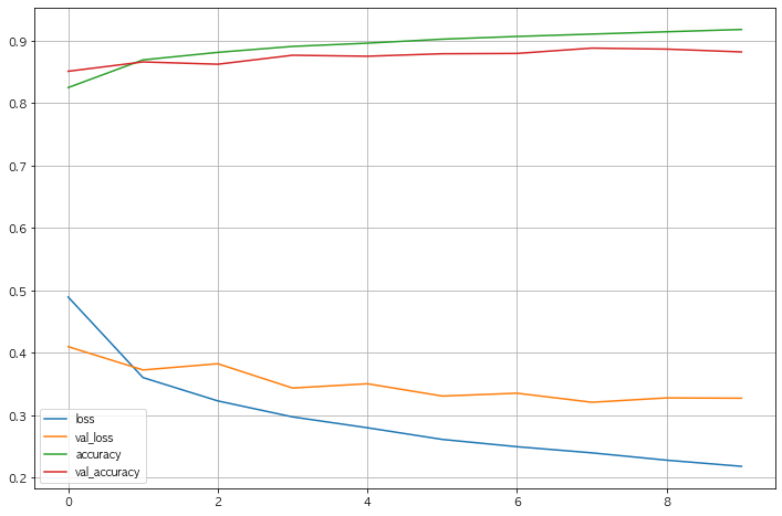
- Acc는 오르고 Loss는 떨어져서 학습이 잘 되는것처럼 보이나 Val Loss와 Loss의 차이가 점점 벌어진다.
3.8 Test Data Acc
1
2
3
score = model.evaluate(X_test, y_test)
print('Test Loss : ', score[0])
print('Test Acc : ', score[1])
1
2
3
313/313 [==============================] - 0s 876us/step - loss: 0.3274 - accuracy: 0.8821
Test Loss :  0.32741284370422363
Test Acc :  0.882099986076355
- Test 데이터는 0.88의 Acc가 나온다
3.9 틀린 데이터 16개 불러와서 그려보기
1
2
3
4
5
import numpy as np

predicted_result = model.predict(X_test)
predicted_labels = np.argmax(predicted_result, axis = 1)
predicted_labels[:10], y_test[:10]
1
2
(array([9, 2, 1, 1, 0, 1, 4, 6, 5, 7]),
 array([9, 2, 1, 1, 6, 1, 4, 6, 5, 7], dtype=uint8))
- 실제 Test 데이터로 예측 후 실제 정답과 비교
1
2
3
4
5
6
wrong_result = []

for n in range(0, len(y_test)):
    if predicted_labels[n] != y_test[n]:
        wrong_result.append(n)
len(wrong_result)
1
1179
- 그중 틀린 데이터만 뽑아옴
1
2
3
4
5
6
7
8
9
10
11
12
import random

samples = random.choices(population= wrong_result, k = 16)
plt.figure(figsize=(14, 12))

for idx, n in enumerate(samples):
    plt.subplot(4, 4, idx + 1)
    plt.imshow(X_test[n].reshape(28, 28), cmap = 'Greys', interpolation='nearest')
    plt.title('Label : ' + str(y_test[n]) + ' Predict : ' + str(predicted_labels[n]))
    plt.axis('off')

plt.show()
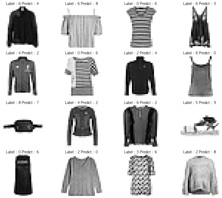
- 레이블 설명
1
2
3
4
5
6
7
8
9
10
0 티셔츠/탑
1 바지
2 풀오버(스웨터의 일종)
3 드레스
4 코트
5 샌들
6 셔츠
7 스니커즈
8 가방
9 앵클 부츠
- 비슷하게 생긴게 좀 많아보인다.
4. 요약
4.1 요약
- 딥러닝의 튜토리얼 MNIST 데이터로 모델을 만들고 예측을 하는 내용이다.
- 딥러닝은 model 생성하는 모델 구조도를 만드는게 어려울것 같다
- 특히나 그 구조도는 만들기 나름이라, 많은 공부가 필요할듯 하다