출처
- https://towardsdatascience.com/3-pandas-functions-that-will-make-your-life-easier-4d0ce57775a1의 블로그를 보고 작성한것 입니다.
1. 들어가면서
- Pandas는 데이터 분석에 있어 널리 사용되는 라이브러리 입니다. 또한 데이터 분석을 위한 다양한 기능과 방법을 제공합니다.
- Pandas에서 유용하게 사용할수 있는 기능을 정리합니다.
2. Convert_dtypes
- 효율적인 데이터 분석을 위해서는 변수에 가장 적합한 데이터 유형을 사용해야 합니다.
- 또한 연산과 같은 일부 기능을 사용하기 위해서는 특정 데이터 유형이 있어야 합니다.
- 특정 상황에서는 문자열 데이터 타입이 객체형 데이터 타입보다 더 선호될수도 있습니다.
- Pandas는 데이터 유형 변환을 처리하는 메서드를 제공합니다.
- Convert_dtypes는 각 개별적 컬럼을 적합한 데이터 유형으로 변환 해줍니다.
- 아래의 Sample Data로 확인해보겠습니다.
- 공식 문서 : https://pandas.pydata.org/pandas-docs/stable/reference/api/pandas.DataFrame.convert_dtypes.html
1
2
3
import numpy as np
import pandas as pd
%matplotlib inline
1
2
3
4
5
6
7
8
9
10
11
12
13
14
name = pd.Series(['John', 'Jane', 'Emily', 'Robert', 'Ashley'])
height = pd.Series([1.80, 1.79, 1.76, 1.81, 1.75], dtype='object')
weight = pd.Series([83, 63, 66, 74, 64], dtype='object')
enroll = pd.Series([True, True, False, True, False], dtype='object')
team = pd.Series(['A', 'A', 'B', 'C', 'B'])

df = pd.DataFrame({
    'name':name,
    'height':height,
    'weight':weight,
    'enroll':enroll,
    'team':team
})
df
| name | height | weight | enroll | team | |
|---|---|---|---|---|---|
| 0 | John | 1.8 | 83 | True | A |
| 1 | Jane | 1.79 | 63 | True | A |
| 2 | Emily | 1.76 | 66 | False | B |
| 3 | Robert | 1.81 | 74 | True | C |
| 4 | Ashley | 1.75 | 64 | False | B |
1
df.dtypes
1
2
3
4
5
6
name      object
height    object
weight    object
enroll    object
team      object
dtype: object
- 위에서 생성한 데이터프레임의 각 열은 모두 object의 데이터 타입을 가지고 있습니다.
1
2
df_new = df.convert_dtypes()
df_new.dtypes
1
2
3
4
5
6
name       string
height    float64
weight      Int64
enroll    boolean
team       string
dtype: object
- convert_dtypes의 메소드를 사용하여 각 열을 알맞은 데이터 타입으로 변환시켜주었습니다.
1
df_new
| name | height | weight | enroll | team | |
|---|---|---|---|---|---|
| 0 | John | 1.80 | 83 | True | A |
| 1 | Jane | 1.79 | 63 | True | A |
| 2 | Emily | 1.76 | 66 | False | B |
| 3 | Robert | 1.81 | 74 | True | C |
| 4 | Ashley | 1.75 | 64 | False | B |
1
2
df_new = df.convert_dtypes(convert_boolean=False)
df_new
| name | height | weight | enroll | team | |
|---|---|---|---|---|---|
| 0 | John | 1.80 | 83 | 1 | A |
| 1 | Jane | 1.79 | 63 | 1 | A |
| 2 | Emily | 1.81 | 66 | 0 | B |
| 3 | Robert | 1.75 | 74 | 1 | C |
| 4 | Ashley | NaN | 64 | 0 | B |
- 또한 conver_boolean의 옵션으로 True, False의 Boolean 데이터 타입도 conver_boolean의 옵션을 False로 주게되면 0과 1로 변환을 시켜주어 분석에 더 용이하게 해준다.
Pipe
- Pipe 함수를 사용하면 체인과 같은 형식으로 많은 작업을 결합 할수 있습니다.
- Pipe 함수는 다른 함수를 입력으로 받으며, 데이터프레임 형식에서 사용 할수 있습니다.
- 공식 문서 : https://pandas.pydata.org/pandas-docs/stable/reference/api/pandas.DataFrame.pipe.html
1
2
3
4
5
6
7
8
9
10
11
12
13
14
name = pd.Series(['John', 'Jane', np.nan, 'Robert', 'Ashley'])
height = pd.Series([1.80, 1.79, 1.76, 1.81, 1.75])
weight = pd.Series([83, 63, 66, 74, 64])
enroll = pd.Series([True, True, False, True, False])
team = pd.Series(['A', 'A', 'B', 'C', 'B'], dtype='string')

df = pd.DataFrame({
    'name':name,
    'height':height,
    'weight':weight,
    'enroll':enroll,
    'team':team
})
df
| name | height | weight | enroll | team | |
|---|---|---|---|---|---|
| 0 | John | 1.80 | 83 | True | A |
| 1 | Jane | 1.79 | 63 | True | A |
| 2 | NaN | 1.76 | 66 | False | B |
| 3 | Robert | 1.81 | 74 | True | C |
| 4 | Ashley | 1.75 | 64 | False | B |
- height는 미터에서 인치로 변환
- Null Data가 있는 행을 삭제
- 문자열 타입의 컬럼을 범주형으로 변경
- 데이터프레임에서 위의 3가지를 변경하겠습니다.
1
2
3
4
5
6
7
8
9
10
11
12
13
14
15
16
17
18
19
# 1. height의 미터를 인치로 변환
def m_to_inch(dataf, column_name):
    # 1m = (1 / 0.0254)
    dataf[column_name] = dataf[column_name] / 0.0254
    return dataf

# 2. Null data는 행 삭제
def drop_missing(dataf):
    dataf.dropna(axis=0, how='any', inplace=True)
    return dataf

# 3. 문자열 타입의 컬럼을 범주형으로 변경
def to_category(dataf):
    cols = dataf.select_dtypes(include='string').columns
    for col in cols:
        ratio = len(dataf[col].value_counts()) / len(dataf)
        if ratio < 0.05:
            dataf[col] = dataf[col].astype('category')
    return dataf
- 위에서 요구한 3가지 사항에 대해 각각 함수를 작성하였습니다.
- 다만 문제는 위의 함수를 모두 적용하면 코드가 길어지고, 가독성이 떨어질것 같습니다.
- 이럴때 Pipe 메소드를 사용하면 편리합니다.
1
2
3
4
5
df_processed = (df.
                pipe(m_to_inch, 'height').
                pipe(drop_missing).
                pipe(to_category))
df_processed
| name | height | weight | enroll | team | |
|---|---|---|---|---|---|
| 0 | John | 70.866142 | 83 | True | A |
| 1 | Jane | 70.472441 | 63 | True | A |
| 3 | Robert | 71.259843 | 74 | True | C |
| 4 | Ashley | 68.897638 | 64 | False | B |
1
df_processed.dtypes
1
2
3
4
5
6
name       object
height    float64
weight      int64
enroll       bool
team       string
dtype: object
- 개별의 함수가 pipe 메소드를 통해서 변경되었습니다.
- 또한 pipe 메소드를 사용하여 코드도 간결하고 가독성이 좋습니다.
1
df
| name | height | weight | enroll | team | |
|---|---|---|---|---|---|
| 0 | John | 70.866142 | 83 | True | A |
| 1 | Jane | 70.472441 | 63 | True | A |
| 3 | Robert | 71.259843 | 74 | True | C |
| 4 | Ashley | 68.897638 | 64 | False | B |
- 주의 : pipe 메소드는 기존의 데이터프레임을 수정합니다. 가능하면 기존의 데이터 프레임의 변경이 없어야 하기 때문에. 원본 데이터 프레임을 다른 사본으로 copy하고 진행하는것이 좋습니다.
- 위의 df라는 데이터프레임을 보면 수정하지 않았지만, pipe가 적용된 모습입니다.
4. Plot
- 판다스는 시각화 라이브러리는 아니지만, 기본적인 시각화 기능은 가지고 있습니다.
- 또한 이러한 시각화 기능흔 다른 시각화 라이브러리에 비해 사용이 간편하고 빠릅니다.
- 공식문서 : https://pandas.pydata.org/pandas-docs/stable/reference/api/pandas.DataFrame.plot.html
1
2
marketing = pd.read_csv('./datas/DirectMarketing.csv')
marketing.head()
| Age | Gender | OwnHome | Married | Location | Salary | Children | History | Catalogs | AmountSpent | |
|---|---|---|---|---|---|---|---|---|---|---|
| 0 | Old | Female | Own | Single | Far | 47500 | 0 | High | 6 | 755 |
| 1 | Middle | Male | Rent | Single | Close | 63600 | 0 | High | 6 | 1318 |
| 2 | Young | Female | Rent | Single | Close | 13500 | 0 | Low | 18 | 296 |
| 3 | Middle | Male | Own | Married | Close | 85600 | 1 | High | 18 | 2436 |
| 4 | Middle | Female | Own | Single | Close | 68400 | 0 | High | 12 | 1304 |
- 위의 Marketing Data를 가지고 실습해보겠습니다.
- 데이터 출처 : https://www.kaggle.com/yoghurtpatil/direct-marketing
1
2
marketing.AmountSpent.plot(kind='hist', title='Amount Spent', figsize=(8,5))
plt.show()
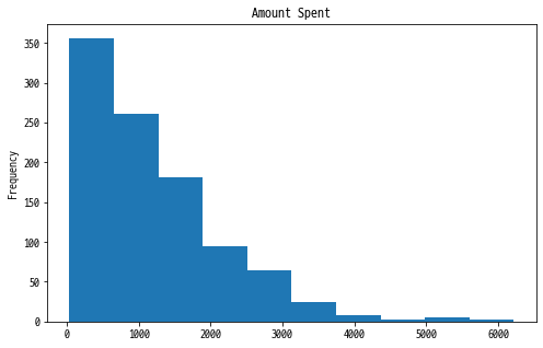
- Amount Spent 컬럼을 plot 메소드를 사용하여 쉽게 확인 가능합니다.
1
2
marketing.plot(x='Salary', y='AmountSpent', kind='scatter', title='Salary VS Amount Spent', figsize=(8,5))
plt.show()
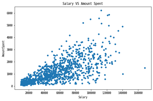
- Salary와 Amount Spent의 관계를 Scatter plot을 사용하여 그려보았습니다.
- 위의 예제 말고도 많은 그래프를 plot 함수를 통해 그릴수 있습니다.
- 이는 다른 시각화 라이브러리를 사용하지않아도 간단한 그래프는 쉽게 그릴수 있습니다.
5. 결론 및 회고
- Pandas의 유용한 3가지 기능을 알아보았습니다.
- Pandas는 데이터분석에 있어 속도도 빠르고, 직관적이며 사용하기 쉬워서 굉장히 많은 사랑을 받는 라이브러리입니다.
- 저도 데이터 분석을 할때 import pandas as pd를 가장 맨위에 적을 정도로 굉장히 많이 쓰고 있습니다.
- Pandas의 더 많은 기능은 아래의 공식 문서를 확인하면 좋을듯 합니다.
- 공식 문서 : https://pandas.pydata.org/pandas-docs/stable/index.html
1